Pima India Diabetes - Modelling with Logistic Regression & Random Forest

In this analysis, we'll find out the major causes for Diabetes. We'll use both logistic regression and Random forest for the analysis. Before getting in to modelling, we have to prepare the data for visualizations and modelling.

#load all the necessary libraries

install.packages("corrplot") install.packages("pROC") install.packages("ROCR")

library(corrplot) library(ggplot2) library(data.table) library(tidyr) library(tm) library(randomForest) library(lattice) library(caret) library(ROCR) setwd("C:/Users/Ed/Desktop/datasets") db = read.csv("diabetes.csv", header=T, na.strings=c("","NA")) View(db)

#pic1

str(db) #=============================================================================================== #Data Preparation #===============================================================================================

cor(db) summary(db) #skinthickness, insulin and bloodpressure has a lot of 0 values. and none of the factors have a linearity #with each other. Therefore we'll have to fill the 0 values with median of each vectors in the #respective columns

db$Outcome = as.factor(db$Outcome) median(db$BloodPressure)#72 median(db$SkinThickness)#23 median(db$Insulin)#30.5 median(db$BMI)#32 median(db$Glucose)#117 #You can get all the values of the median from the summary table also.

db$BloodPressure = ifelse(db$BloodPressure==0,72,db$BloodPressure) db$SkinThickness = ifelse(db$SkinThickness==0,23,db$SkinThickness) db$Insulin = ifelse(db$Insulin==0,30.5,db$Insulin) db$BMI = ifelse(db$BMI==0,32,db$BMI) db$Glucose = ifelse(db$Glucose==0,117,db$Glucose)

View(db)

#pic2

cor(db) gg = symnum(cor(db[,-9], use = "complete.obs")) corr = cor(db[,-9]) # compute correlation matrix corrplot(corr, method="square")

#pic3

#There are still no linearity between the factors.

#creating age groups

db$age_group=cut(db$Age, breaks = c(0, 5, 10, 15, 20, 25, 30, 35, 40, 45, 50, 55, 60, 65, 70, 85, 100, 115), labels = c("0-5", "6-10", "11-15", "16-20", "21-25", "26-30", "31-35", "36-40", "41-45", "46-50", "51-55", "56-60", "61-65", "66-70", "71-85", "86-100", "101-115" )) # grouping the ages using break function

View(db) str(db$age_group)

#=============================================================================================== #Visulaizations #===============================================================================================

ggplot(data = db, aes(x=age_group))+geom_bar(stat = "count", fill = "purple") + theme_bw() + xlab("age group") + ylab("Count") + ggtitle("Age group statistics") + theme(plot.title = element_text(hjust = 0.5))

#pic4

ggplot(data = db, aes(x = age_group, fill = Outcome)) + geom_bar(stat="count") + theme_bw() + xlab("age group") + ylab("Outcome") + ggtitle("Age group Outcome statistics") + theme(plot.title = element_text(hjust = 0.5))

#pic5

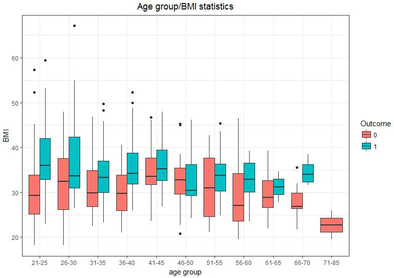
ggplot(data = db, aes(x= age_group, y = BMI, fill = Outcome))+ geom_boxplot()+ theme_bw() + xlab("age group") + ylab("BMI") + ggtitle("Age group/BMI statistics") + theme(plot.title = element_text(hjust = 0.5))

#pic6

ggplot(data = db, aes(x= age_group, y = Pregnancies, fill = Outcome))+ geom_boxplot()+ theme_bw() + xlab("age group") + ylab("Pregnancies") + ggtitle("Age group/Pregnancies statistics") + theme(plot.title = element_text(hjust = 0.5))

#pic7

ggplot(data = db, aes(x= age_group, y = BloodPressure, fill = Outcome))+ geom_boxplot()+ theme_bw() + xlab("age group") + ylab("BloodPressure") + ggtitle("Age group/BloodPressure Statistics") + theme(plot.title = element_text(hjust = 0.5))

#pic8

ggplot(data = db, aes(x= age_group, y = SkinThickness, fill = Outcome))+ geom_boxplot()+ theme_bw() + xlab("age group") + ylab("Skin thickness") + ggtitle("Age group/Skin thickness statistics") + theme(plot.title = element_text(hjust = 0.5))

#pic9

ggplot(data = db, aes(x= age_group, y = Insulin, fill = Outcome))+geom_boxplot()+ theme_bw() + xlab("age group") + ylab("Insulin") + ggtitle("Age group/Insulin statistics") + theme(plot.title = element_text(hjust = 0.5))

#pic10

ggplot(data = db, aes(x= age_group, y = Glucose, fill = Outcome))+geom_boxplot()+ theme_bw() + xlab("age group") + ylab("Glucose") + ggtitle("Age group/Glucose statistics") + theme(plot.title = element_text(hjust = 0.5))

#pic11

#Predictive Modelling

#========================================================================================= #Modelling using Logistic Regression #=========================================================================================

dbnew = db[,-c(10)] str(dbnew)

set.seed(123) ind = sample(2, nrow(dbnew), replace = TRUE, prob = c(0.7,0.3)) train = dbnew[ind==1,] test = dbnew[ind==2,]

glm1 = glm(Outcome~.,data = train, family = "binomial") coefficients(glm1) summary(glm1)

glm2 = glm(Outcome~Pregnancies+Glucose+Insulin+BMI+DiabetesPedigreeFunction, data = train, family = "binomial") summary(glm2)

predmain = predict(glm1, test, type = "response")

pred = predict(glm2, test, type = "response") pred

head(test)

pred[3] #probability = 0.83, actual outcome is 1 (prob > 0.5 => outcome will be 1, we are going by this intuition) pred[2] #probability = 0.036, actual outcome is 0 pred[1] #probability = 0.034, actual outcome is 0

#Above we tested the predicted value with the actual outcome and it turned out that # our predictions are true for all 3 of the cases. Although it might not be the case #for all the observations. There are chances of errors.

#Therefore, we have to create a confusion matrix to find the misclassification error

#Misclassification error

#with the first model with all the independent variables(glm1) modelpred1 = rep("0",229) modelpred1[predmain>0.5] = "1" tab1 = table(modelpred1,test$Outcome) print(tab1)#confusion matrix 1-sum(diag(tab1))/sum(tab1)

#0.2620 is the misclassification error

#second model with two independent variables removed (glm2) modelpred = rep("0",229) modelpred[pred>0.5] = "1" tab = table(modelpred,test$Outcome) print(tab) #confusion matrix 1-sum(diag(tab))/sum(tab)

#0.2532 is the classification error ( A model with the mower misclassification error is selected as the model)

#Therefore we have found out that glm2 is the better model of the two.

#Plotting are under ROC Curve for logistic regression #=========================================================================================

predaoc = predict(glm2,type = c("response"))

train$predaoc = predaoc aoc1 = roc(Outcome~predaoc, data = train) plot(aoc1)

#Now we'll perform the randomforest modelling on the training data set 'train'

#===================================================================================== # Modelling using Random Forest #=====================================================================================

rf1 = randomForest(Outcome ~ Pregnancies+Glucose+Insulin+BMI+DiabetesPedigreeFunction, data = train) print(rf1)

rf1$confusion

pred1 = predict(rf1, train) head(pred1) head(train$Outcome)

#The first 6 predictions are true, nothing but coincidence. This cannot be the case all the time #We have out of bag error of 23%. We'll further dig deep on this in the following steps.

confusionMatrix(pred1, train$Outcome)

pred2 = predict(rf1,test)

confusionMatrix(pred2, test$Outcome)

plot(rf1)

t1 = tuneRF(train[,-9], train[,9], stepFactor = 0.5, plot = TRUE, ntreeTry = 500, trace = TRUE, improve = 0.05) #mtry = 3

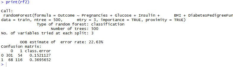
rf2 = randomForest(Outcome~Pregnancies+Glucose+Insulin+BMI+DiabetesPedigreeFunction, data = train, ntree = 500, mtry = 3, importance = TRUE, proximity = TRUE) print(rf2)

print(rf1)

pred3 = predict(rf2,test)

confusionMatrix(pred3, test$Outcome)

confusionMatrix(pred2, test$Outcome)

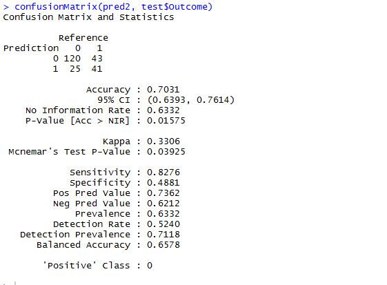
When the above two confusion matrices are compared, you can see the increase in the accuracy in the tuned rf model. Therefore it is evident that the tuned random forest model 'rf2' is more accurate than the first random forest model 'rf1'.

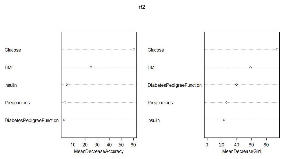
varImpPlot(rf2)

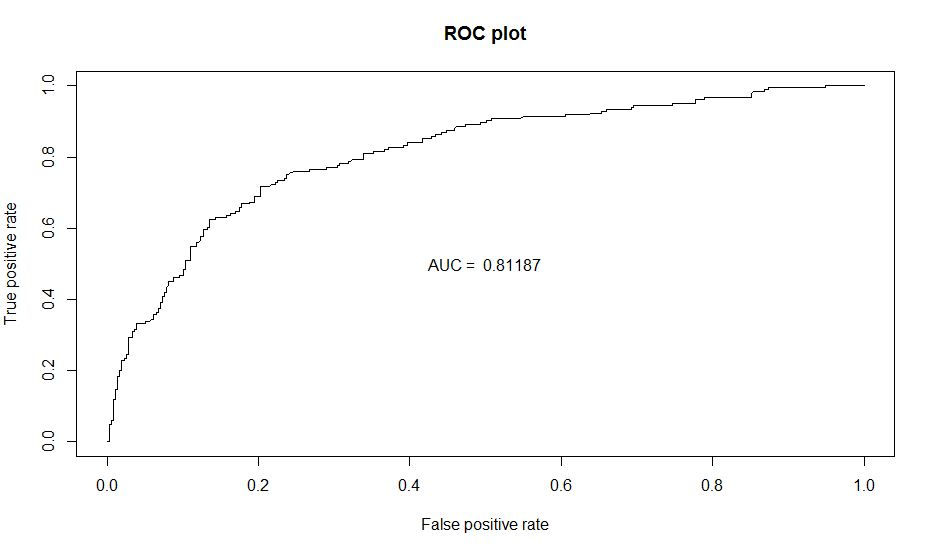
#Plotting are under ROC Curve for Random forest #=========================================================================================

predictions = as.vector(rf2$votes[,2]) predd = prediction(predictions,train$Outcome)

perfauc = performance(predd,"auc") AUC=perfauc@y.values[[1]]

perf_ROC=performance(predd,"tpr","fpr") #plot the actual ROC curve plot(perf_ROC, main="ROC plot") text(0.5,0.5,paste("AUC = ",format(AUC, digits=5, scientific=FALSE)))

Conclusion

Highlights:

Glusose has directly proportional affect on the diabetes outcome. In the importance plot of the random forest model, you can see that Glucose followed by BMI has the most importance. In the logistic regression model, again Glucose and BMI has the most significance. Rest of the inferences can be obtained from the visualizations itself.

23.75% is the out of the bag error for the first random forest model 'rf1' and 22.63% is the OOB for the tuned model and accuracy has seen an increase in the test data as well.